PyMol & Multiwfn Electrostatic Potential (ESP) Visualization
Generate ESP .cub file from the Multiwfn and plot it in PyMol
Related Multiwfn Documents
http://sobereva.com/443
http://sobereva.com/196Related PyMol Documents
https://pymolwiki.org/index.php/Ramp_New
Generate .fchk file with Gaussian
- Run a single point calculation and save the wavefuncation information to the .chk file
%chk=xxx.chk - Make the formchk file and refine it with sed. (Make it readable to GaussView)
for i in *.chk; do formchk $i ${i%chk}fchk && sed -i 's/MM charges/MM charge /g' ${i%chk}fchk && sed -i 's/MicOpt/Opt /g' ${i%chk}fchk; done
Generate .cub file with Multiwfn
Single file
- set the cubegen path in $Multiwfn_HOME/setting.ini
This greatly accelerate the calculation - open Multiwfn.exe
- load the .fchk file
- Run ESP calculation
The following numbers are the Multiwfn control-indexHere we got the .cub file for ESP isosurface5 # Output and plot specific property within a spatial region (calc. grid data)
1 # Electron density
2 # Medium quality grid, covering whole system
2 # Export data to Gaussian-type cube file in current folderdensity.cubHere we got the .cub file for ESP color mapping0 # Return to main menu
5 # Output and plot specific property within a spatial region (calc. grid data)
12 # Total electrostatic potential (ESP)
1 # Low quality grid , covering whole system
# Running: "cubegen 4 potential=SCF xxx.fchk ESPresult.cub -1 h ESPgridtmp.cub > nouseout"
2 # Export data to Gaussian-type cube file in current foldertotesp.cub
Multiple file
A .bat/.ps1 file can help dealing with multiple .fchk
Multiwfn XXX.fchk < ESPiso.txt |
The .txt file contain the control-index listed above
Visualize the surface with PyMol
- open the structure (save a .mol2 from any of the .cub) and these two .cub files
- Use “Other Visualization Settings for structures” from https://www.shaoqz.cn/2020/06/29/PyMol-Orbital/
- Build IsosurfaceGrammer: isosurface {new object name}, {.cub name}, {isovalue}
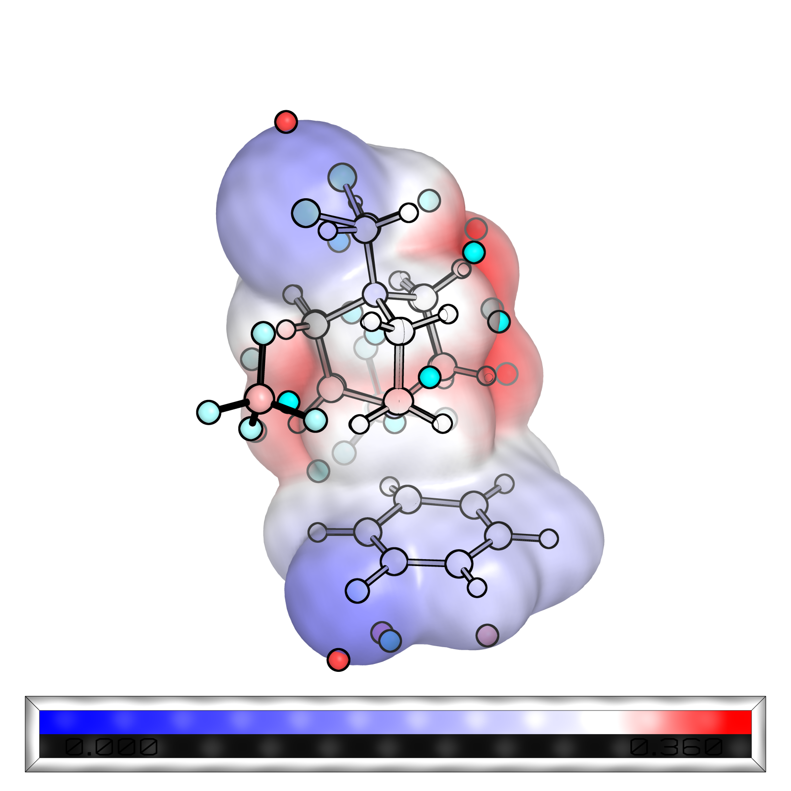
isosurface ESP1, density, 0.002
set transparency, 0.2 - Color the surface with ESPGrammer: ramp_new {new object name}, {ESP .cub name}, [Value list], [Corresponding color list]
ramp_new ramp1, totesp, [0, 0.3, 0.36], [blue, white, red]
color ramp1, ESP1
Grammer: color {color object}, {object}
The extreme point analysis
In Multiwfn with the .fchk loaded
12 # Quantitative analysis of molecular surface |
Maxima is presented as carbon
Minima is presented as oxygen